


The cavity model is a descriptive name we gave to the NM-64 design as it relies on cavities created by Pb rings in which moderated thermal neutron detectors (typically BP-28 BF\(_3\) counters) are located (Fig. 1a). Incoming CR nucleons, for the most part, pass through the outer polyethylene reflector material unperturbed. The purpose of the outer reflector is to shield and absorb the low energy neutrons that are produced by high-energy nucleonic interactions with the materials surrounding the monitor. A CR nucleon that passes through the reflector then may undergo a violent nuclear reaction (known as spallation) with the heavy Pb nucleus of the producer material. In the context of the present discussion, spallation occurs when a relativistic light, but very high-energy particle (a proton or a neutron) hits a heavy nucleus causing it to disintegrate through inelastic nuclear reactions. The disintegration of the Pb nuclei results in the emission of neutrons and other particles, essentially amplifying the response to be measured. The reflector material has a dual function, as well as isolating from environmental influences, it moderates and reflects the neutrons produced by the reactions in the Pb producer inwards towards the neutron detectors. Neutrons generated during the spallation reaction are then thermalised by the polyethylene moderator surrounding the thermal neutron detectors. The thermal neutrons are then detected indirectly by ionising particles that are produced in a neutron induced nuclear reaction (for detectors employing BF\(_3\), thermal neutrons captured in the \(^10\)B are converted into secondary particles through the \(^10\)B(n,\(\alpha\))\(^7\)Li reaction, while detectors employing \(^3\)He, thermal neutrons are converted into secondaries through the \(^3\)He(n,p)\(^3\)H reaction).
The slab model, presented here for the first time, describes a configuration of reflector, producer and moderator arrangement that resembles a slab (Fig. 5), i.e., it eliminates the producer and moderator rings employed by the cavity model. Instead, a cuboidal polyethylene moderator slab with uniformly distributed detectors (received via machined bores in the moderator) is encased in a cuboidal Pb sarcophagus before being encased in an outer layer of polyethylene reflector. This affords greater flexibility, simplifies fabrication (so reduces cost) and increases the sensor packing density by eliminating the voids inherent in the cavity model. The slab concept still relies on the fundamental detection physics of the NM-64 (cavity) design.
NM-64 benchmark
To establish a modelling benchmark, a 6-NM-64 radiation transport model was developed based on the reported design parameters20. A CAD model was first devised in Ansys ® SpaceClaim42, with material types classified by colour. The model conformed to constructive solid geometry without any modifications and was subsequently converted into MCNP geometry. The integrity of the translated geometry was tested for lost particles using a void run and zero lost particles were identified in 10\(^9\) source particles, indicating a well defined geometry for radiation transport calculation. Figure 1a shows a vertical cross section of the 6-NM-64 benchmark model. A benchmark count rate was derived using the 6-NM-64 model and source term (detailed in the “Methods”), running for \(10^7\) source particle histories with results presented in Table 1.
NM-64 equivalent comparisons
To create a 6-NM-64 equivalent using the parameterised cavity model (Fig. 1b and described in the “Methods” section), the 6-NM-64 dimensions20 were used to determine values for the cavity radius (\(r\_cavity\)), the inner moderator thickness (\(t\_mod\)), the air gap thickness (\(t\_air\)) and the outer moderator thickness (\(t\_box\)). In the cavity model, the wings of the Pb rings were omitted from the standard NM-64 design, a producer thickness (\(t\_prod\)) value was calculated such that an equivalent producer mass is conserved between the 6-NM-64 benchmark and equivalent cavity model. The producer mass in the benchmark 6-NM-64 is 9650 kg20, corresponding to a \(t\_prod\) value of 6.77 cm in the equivalent model.
The equivalent model was ran for 10\(^7\) source particles and compared to the benchmark model. The output data are compared in Table 1, the statistical errors on the total count rate for both models overlap, indicating that removing the wings from the NM-64 benchmark design is statistically negligible. To simplify the engineering of any potential cavity based design, the wings could therefore be removed from the design. The wings were originally included to provide a uniform Pb thickness for use with a meson monitor placed below it, making use of the Pb as a soft component absorber (our slab design achieves this naturally)20.
In considering BCS-based detectors as an alternative to the BF\(_3\) counters used in the original NM-64, multiple 1\(^\prime \prime \) dia. PTI-204 BCS detectors41 were modelled in the cavity of the 6-NM-64 equivalent model. The PTI-204 detector is made up of seven round 7.5 mm diameter boron coated straws encased in a 1\(^\prime \prime \) dia. aluminium tube. Each straw element in the PTI-204 detector represents mini proportional counters. Straws are tied together to give one signal output and supplied with an integrated amplifier and high voltage supply43,44. The BCS tubes were extended to the same length as the BF\(_3\) counters to provide a direct comparison. Simulations were ran for 1, 7 and 19 tubes per cavity to count surplus thermal neutron production which may exist within the cavity. The 1, 7 and 19 tube configurations are shown in Fig. 2a,c,e, respectively.
Table 1 compares the relative count rate for the NM-64 equivalent cavity model with 1, 7 and 19 PTI-204 BCS tubes per cavity against the 6-NM-64 benchmark data, each simulation was ran for \(10^7\) source particles. The relative count rate increase drops off as a function of the number of tubes per cavity, for example, the count rate for 7 tubes per cavity is less than 7 times higher than 1 tube per cavity. The count rate achieved with 19 tubes per cavity exceeds the benchmark 6-NM-64 count rate by a statistically significant margin. However, when considering the spatial distribution of reaction rate per unit volume (Fig. 2b,d,f), the 19 tube configuration (Fig. 2e) does not appear to be the optimum use of those detectors; intense yellow indicating a high relative reaction rate, dark blue indicating a low (depleted) reaction rate. Here a neutron mesh tally was calculated over the full detector, with a \(^10\)B(n,\(\alpha\)) reaction rate tally multiplier applied to the mesh. The results therefore provide an indicative spatial distribution of neutron detection probability, which is directly proportional to the \(^10\)B(n,\(\alpha\)) reaction rate. Figure 2b,d,f shows that a potentially higher reaction rate in some of the tubes could be achieved if they were moved elsewhere in the assembly, thus the 19 tube per cavity configuration is sub-optimal.
Randomised parameter scan
To explore the full parameter space of the parameterised cavity model, parameters were randomly generated within specified ranges (shown in Table 2) to construct 1000 unique models for the BP28-BF\(_3\) counter. Fig. 1c shows the resulting scatter plot of the producer mass against the total count rate. The 6-NM-64 baseline count rate (43.04 cnts s\(^-1\)), indicated by the orange marker, is exceeded by many of the configurations derived. However, only 7 of these have a lower Pb mass than the 6-NM-64 standard, which indicates a well optimised NM-64 configuration and prompted our investigations into alternative slab configurations.

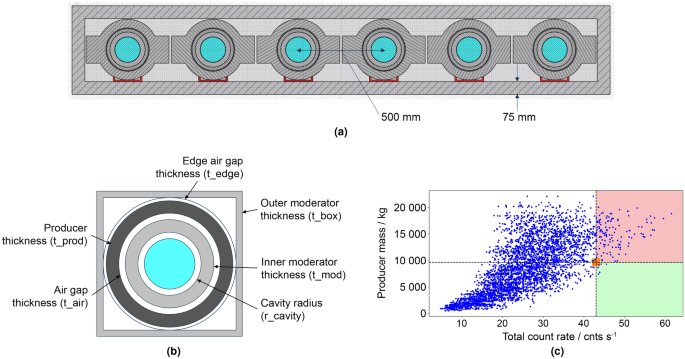
6-NM-64 parameterisation. (a) Vertical cross section (to scale) of the radiation transport model developed and used to represent the 6-NM-64 benchmark. Moving from the inside out, comprising six 6\(^\prime \prime \) dia. BP28-BF\(_3\) proportional counters (blue), air gap, 2 cm thick HDPE moderator tube and 5.1 cm thick winged Pb rings (one per counter) and outer 7.5 cm thick HDPE reflector with dimensions as indicated. (b) Single counter representation of the parameterised cavity model used as an equivalent to the NM-64 standard with key parameters indicated. NB: this figure represents a single cavity; all simulation performed in this study were for six cavities as per the 6-NM-64 benchmark. The wings of the Pb rings were omitted from the standard NM-64 design for simplicity. (c) Producer mass in kg against total (i.e., summed across all six detectors) count rate in cnts s \(^-1\) for randomly generated parameter configurations of the parameterised cavity model shown in (b). The orange marker, located at the intercept of the orthogonal dashed lines, indicates the 6-NM-64 benchmark performance; a count rate of \(\sim\)43 cnts s\(^-1\) for a producer mass of \(\sim\)10 tonne. The region shaded red signifies parameter configurations that exceed the count rate performance of the 6-NM-64 benchmark but for a greater producer mass. The region shaded green signifies parameter configurations that exceed the count rate performance of the 6-NM-64 benchmark but for a lower producer mass. The few parameter configurations in the region shaded green indicates a well optimised NM-64 configuration.

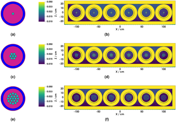
NM-64 equivalent parameterised cavity model filled with (a) 1, (c) 7 and (e) 19 PTI-204 BCS detectors per cavity. Indicative spatial distribution of the \(^10\)B(n,\(\alpha\)) reaction rate tally with (b) 1, (d) 7 and (f) 19 PTI-204 BCS detectors per cavity. Intense yellow indicating a high relative reaction rate, dark blue indicating a low (depleted) reaction rate.
Slab parameter optimisation
To determine the potential neutron detection efficiency of a given slab configuration (shown in Fig. 8a), a cell tally was added to the moderator block, with a \(^10\)B(n,\(\alpha\)) reaction rate tally multiplier added. Whilst this is not a direct measure of neutron detection efficiency, the global reaction rate calculated within the moderator provides a basic figure of merit (FOM) and relates to the potential efficiency. The FOM is defined by Eq. (1). Using this, three separate parameter studies were carried out to optimise the slab parameters; constant volume, equal Pb thickness and constant Pb mass. For all of these simulations, a 1 m active length detector was assumed.
$$\beginaligned FOM = N_B_4C \cdot V_B_4C \int ^\infty _0 \sigma _B_4C(E) \cdot \phi (E) \cdot dE \endaligned$$
(1)
where \(N_B_4C\) is the number density of boron carbide inside the BCS (assuming 96% \(^10\)B enrichment). \(V_B_4C\) is the volume of boron carbide inside each BCS. \(\sigma _B_4C(E)\) is the total absorption cross section for the boron carbide (\(\gg\)99% of this is the \(^10\)B(n,\(\alpha\)) reaction). \(\phi (E)\) is the average flux over the full inner moderator volume. The integral is directly computed in MCNP and the multiplier outside the integral is the quantity we define as the tally normalisation factor. The FOM is directly related to the count rate we would measure on an individual BCS, however it is based on the average flux over the entire inner moderator slab. Local variations in reaction rate are determined later using the mesh-based approach.
Table 3, column (A), presents the fixed and varied parameters for the constant slab volume simulations, the cross sectional area of the moderator is constrained to equal the internal cross sectional area of the baseline 6-NM-64 (296 cm \(\times\) 39 cm). 500 simulations were performed, with an upper limit of 4 m for the width and 2 m for the height, the aspect ratio was varied between these limits. Figure 3a shows a plot of a FOM (i.e., indicative of the count rate from the \(^10\)B(n,\(\alpha\)) reaction rate tally) against the aspect ratio.

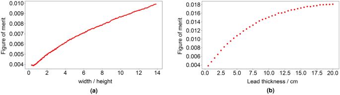
Results of the initial slab parameter optimisations showing the figure of merit (FOM, i.e., the indicative count rate from the \(^10\)B(n,\(\alpha\)) reaction rate tally) against (a) the aspect ratio for all constant volume simulations and (b) the Pb thickness in cm for all equal Pb thickness simulations.

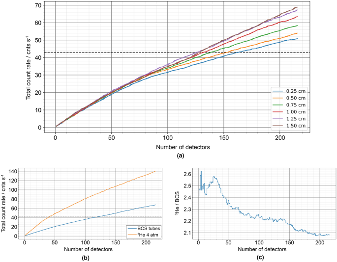
Results of the detector location optimisation simulations within the parameterised slab model showing calculated total count rate in cnts s−1 against (a) number of PTI-204 BCS detectors added for all \(t\_gap\) simulations performed and (b) number of 4 atm \(^3\)He and PTI-204 BCS detectors for \(t\_gap\) = 1.25 cm. The dashed horizontal line shows the 6-NM-64 benchmark count rate for comparison. (c) Shows the ratio of \(^3\)He / BCS total count rate against number of detectors for \(t\_gap\) = 1.25 cm.
The largest aspect ratio yields the greatest count rate. On this basis, fixed parameter values for the equal Pb thickness simulations are given in Table 3, column (B). Here the parameters corresponding to the Pb box geometry shown in Fig. 8a, i.e., the topside (\(t\_prod\)), the side (\(t\_sides\)) and the underside (\(t\_base\)) thickness of the Pb producer, are set equal each other and are then varied from 0.5 to 20.0 cm in intervals of 0.5 cm. Figure 3b shows a plot of the FOM against Pb thickness.
As observed in Fig. 1c, the count rate increases as Pb mass increases. However, the relationship is non-linear as illustrated by Fig. 3b, the rate of count rate increase slows significantly beyond \(\sim\)10 cm.
For the next parameterisation study, a Pb mass of 10000 kg was used, a round figure derived from the perceived optimal 10 cm thickness. Fixed parameter values are given in Table 3, column (C). Keeping the Pb mass constant, \(t\_prod\), \(t\_side\) and \(t\_base\) were varied to determine the optimal ratios to best utilise the given Pb mass. \(t\_base\) was incremented on an inner loop of length 22, from 0.5 to 9.93 cm, where 9.93 cm has been calculated from \(t\_base\) = \(t\_side\) = \(t\_prod\) = 10000 kg of Pb. \(t\_side\) was incremented on an outer loop of length 22, from 0.5 to 9.93 cm, a total of 484 simulations (22 \(\times\) 22).
Further parameterisations derived an optimal ratio of 0.7 (\(t\_base\)) : 0.9 (\(t\_side\)): 1 (\(t\_prod\)). However, the absolute producer mass has more impact on the FOM than its spatial distribution around the inner moderator block.
Detector location optimisation
Using the optimal slab parameters derived, the original cell tally used on the inner moderator block was replaced with a 5 cm resolution mesh tally in width and height, with the same \(^10\)B(n,\(\alpha\)) reaction rate tally multiplier added. This modification allows for local FOM determination within the moderator slab, which can be utilised to inform the optimal location within the moderator to position a neutron detector. An automated process was developed to populate the moderator with neutron detectors in optimal locations. The population methodology is illustrated in Fig. 8b,c. An integrated model generation and output data interpretation process was developed, utilising a mesh tally file reader to process the output data from each iteration. This allowed the maximum voxels not already occupied with a neutron detector to be identified and a detector to be placed in that location in the next iteration.
Iterations were performed for up to 216 neutron detectors on a 400 cm \(\times\) 20 cm \(\times\) 100 cm moderator block. Fixed parameters for all simulations were derived from the analysis described thus far and are defined in Table 3, column C, with repeated iterations carried out for an air gap thickness (\(t\_gap\)) between the outer reflector and the producer, and the producer and the inner moderator (see Fig. 8a) of 0.25 to 1.50 cm in 0.25 cm intervals, a total of 216 \(\times\) 6 simulations.
The count rate distribution across the detectors was found to be more even for the 1.5 cm gap than for the 0.25 cm gap case. This effect is likely due to over moderation in the 0.25 cm gap case; neutrons which enter the detector from above undergo significant moderation, i.e., the mean free path is much shorter than the height of the moderator, and are subsequently mainly absorbed by the top row of detectors. In the 1.5 cm gap case, neutron absorption by the moderator appeared much lower, therefore the overall efficiency of the individual detectors appears to be greater, given that only 129 detectors were required to match the 6-NM-64 performance compared to 164 detectors for the 0.25 cm gap case. In both cases, the preferential location for the addition of neutron detectors appears to be the top row, which implies the optimal geometry would be thinner than that used for these simulations.
From Fig. 4a, the impact of increasing the gap size is shown for an increasing number of detectors; beyond 50 detectors, the increase in count rate observed for smaller gap sizes appears to be less than observed for larger gap sizes. For a similar count rate to the 6-NM-64 benchmark (marked with a black dotted line), 1.25 cm appears the optimum gap size; with this gap size, a count rate of 10 cnts s\(^-1\) more is observed for the same number of detectors added with a gap size of 0.25 cm.
Assuming 1.25 cm as the optimum gap size and retaining the fixed parameters defined in Table 3, column C, a comparative study was performed between the 1\(^\prime \prime \) dia. PTI-204 BCS and an equivalent \(^3\)He detector at 4 atm fill pressure. Figure 4b shows a plot of the total count rate against number of detectors for the PTI-204 BCS and the \(^3\)He detectors. Figure 4c shows a plot of the ratio of \(^3\)He to BCS count rates against number of detectors.
Figure 4b shows an initial steeper count rate increase for the \(^3\)He detectors in up to around 40 detectors, with a slower rate of increase beyond this. By comparison, the BCS count rate increase appears more linear. The key result is the ratio between the \(^3\)He and BCS count rates illustrated in Fig. 4c, which initially peaks to around 2.6 during the initial \(^3\)He count rate increase described and remains above 2 for all detectors added. Comparing the efficiency per detector added (Fig. 3b), the factor of increase from BCS to \(^3\)He approaches 3 for 150 BCS tubes against 50 \(^3\)He tubes (rounded-up tube numbers which achieve a count rate greater than the 6-NM-64 benchmark).
Despite the higher cost of \(^3\)He, the potential design benefits of higher efficiency outweighs the additional cost per detector when considering all cost implications (e.g., additional Pb, polyethylene and electronics to accommodate a greater number of detectors) and long term (>50 years) operating potential. Building on this, detector characteristics that influence relative efficiency (and cost) were considered in achieving optimum efficiency/cost. BCS efficiency inherently depends on the B\(_4\)C deposit thickness, whereas \(^3\)He efficiency is dictated by gas fill pressure. The details of this study are not included here, but based on a detailed engineering breakdown and trade-off arguments, \(^3\)He at 4 atm fill pressure is most cost-effective41.
\(^3\)He detector optimisation
Given the higher detection efficiency of \(^3\)He versus BCS, and therefore an overall smaller instrument size, further parameter optimisations were conducted to maximise the count rate per unit mass of producer for a fixed number of detectors. 50 1 m-long \(^3\)He detectors at 4 atm were chosen (from Fig. 4b, 44 \(^3\)He detectors equals the 6-NM-64 benchmark count rate). Figure 5a presents a visualisation of these parameter optimisations, which included the spacing between detectors, the air void thickness around the detector, the outer reflector box thickness and the air gap between the reflector and Pb producer. Parameters were optimised in order of predicted impact each would have on the overall detection efficiency (i.e., the most significant was optimised first and so on), the principle being that the less significant parameters would act only as fine tuning of the model. The Pb producer thicknesses were retained from the previous BCS optimisations, using \(t\_base\) = 7 cm, \(t\_side\) = 9 cm and \(t\_prod\) = 10 cm. Iteration results are presented in Table 4, with a CAD representation of the optimised model presented in Fig. 5b,c.

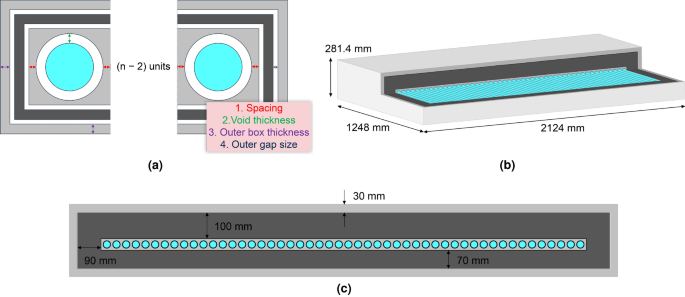
(a) Schematic of the parameterised slab model used for the \(^3\)He detector optimisations. 50 tubes were used for these simulations, the additional 48 tubes present in the centre of the model have been omitted for clarity. Parameters optimised included: 1. the spacing between detectors, 2. the air void thickness around the detector, 3. the outer reflector box thickness and 4. the air gap between the reflector and Pb producer. Parameters were optimised in order of predicted impact each would have on the overall detection efficiency. (b) Cutaway isometric (to scale) of the \(^3\)He optimised model with key dimensions as indicated. (c) Vertical cross section (to scale) of \(^3\)He optimised model with key dimensions as indicated.
\(^3\)He detector optimisation input parameters and output dimensions and specific count rates.
Engineering optimisations
The optimised model was evaluated and analysed by mechanical engineers to derive at a final design that is practical, cost effective and that can be manufactured easily. Figure 6 presents the engineered design solution.

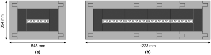
Modular engineered design solution with concessions applied, showing two of the possible four configurations with key dimensions indicated in mm. Following the nomenclature x-NM-2023, where x is the number of banks of six 1\(^\prime \prime \) dia. \(^3\)He detectors and 2023 being the year designed, (a) the quarter-size monitor comprising of 1 bank of six detectors (1-NM-2023) and (b) the full-size monitor comprising of 4 banks of six detectors (4-NM-2023).
The most significant design concession was the use of 2 m long (nominal) \(^3\)He detectors (Reuter-Stokes RS-P4-0878-201)45 rather than the 1 m long detectors used during the optimisations. However, the producer mass (which is shown here to have the most influence over count rate performance) was conserved, essentially halving the width (and number of detectors) and doubling the depth (and length of detectors) with anticipated minimal impact from a neutronics perspective. In engineering terms, this concession halved the number of readout channels, reducing cost and complexity. To fulfil a requirement to modularise the design, 25 detectors were reduced to 24. This allowed detectors to be grouped into four banks of six detectors, providing an even number of detectors per bank and allowing detectors to be paired to a single preamplifier, again reducing cost and complexity. Figure 6a shows a quarter sized monitor and Fig. 6b shows a full size monitor design to equal the count rate of a 6-NM-64 and how the modularisation is achieved in quarter increments. All bulk material components were also modularised for ease of handling and installation, each with a mass <35 kg. The few millimetre gaps between the Pb producer and moderator, and reflector and producer were eliminated to reduce engineering complexities and cost. The analysis presented indicates that this will have minimal impact on performance. The outer reflector thickness was also increased to 7 cm following further analysis, making it equal to the thickness used by the NM-64.
link